In Cableizer the approximate temperature distribution can be calculated by using the superposition principle with image sources or the finite element method using Dirichlet boundary conditions for soil surface and natural boundary conditions in depth.
Posted 2026-01-02
Categories:
Theory
In Cableizer the approximate temperature distribution can be calculated by using one of two options:
We want to discuss the option 1. It is calculated using the formula shown below. The logarithmic term represents the temperature distribution from point heat sources using the method of images.
$$\theta(x,y)=\theta_a+\frac{\rho_4}{2\pi}\sum\limits_{k=1}^N \left\{W_k\ln\left(\frac{\sqrt{(x-x_k)^2+(y+y_k)^2}}{\sqrt{(x-x_k)^2+(y-y_k)^2}}\right)\right\}$$The parameter $\theta_a$ is the ambient temperature (ground surface), $\rho_4$ is the thermal resistivity of the soil, $W_k$ which is the heat source strength (thermal energy) of the k-th point source, $x$ and $y$ the coordinates with $y = 0$ being at the ground surface.
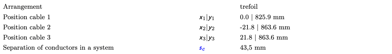
There are three cables in touching trefoil arrangement in a burial depth of 85 cm.
| Arrangement with cables in trefoil | Arrangement with equivalent heat source |
|---|---|
 |
 |
The ambient temperature $\theta_a$ is 15°C, the thermal resistivity of the soil is $\rho_4$ is 1.0 K.m/W
The total losses of the arrangement of the three touching 20 kV cables with 240&mm2 Al operated at 90°C is 98.5 W/m – about 33 W/m per cable. The losses are not the same for these three cables, the upper cable has slightly lower losses.
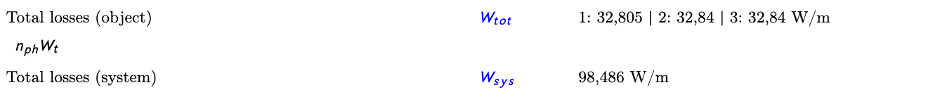

Using the formula above we have to calculate 3 heat sources at three different positions.

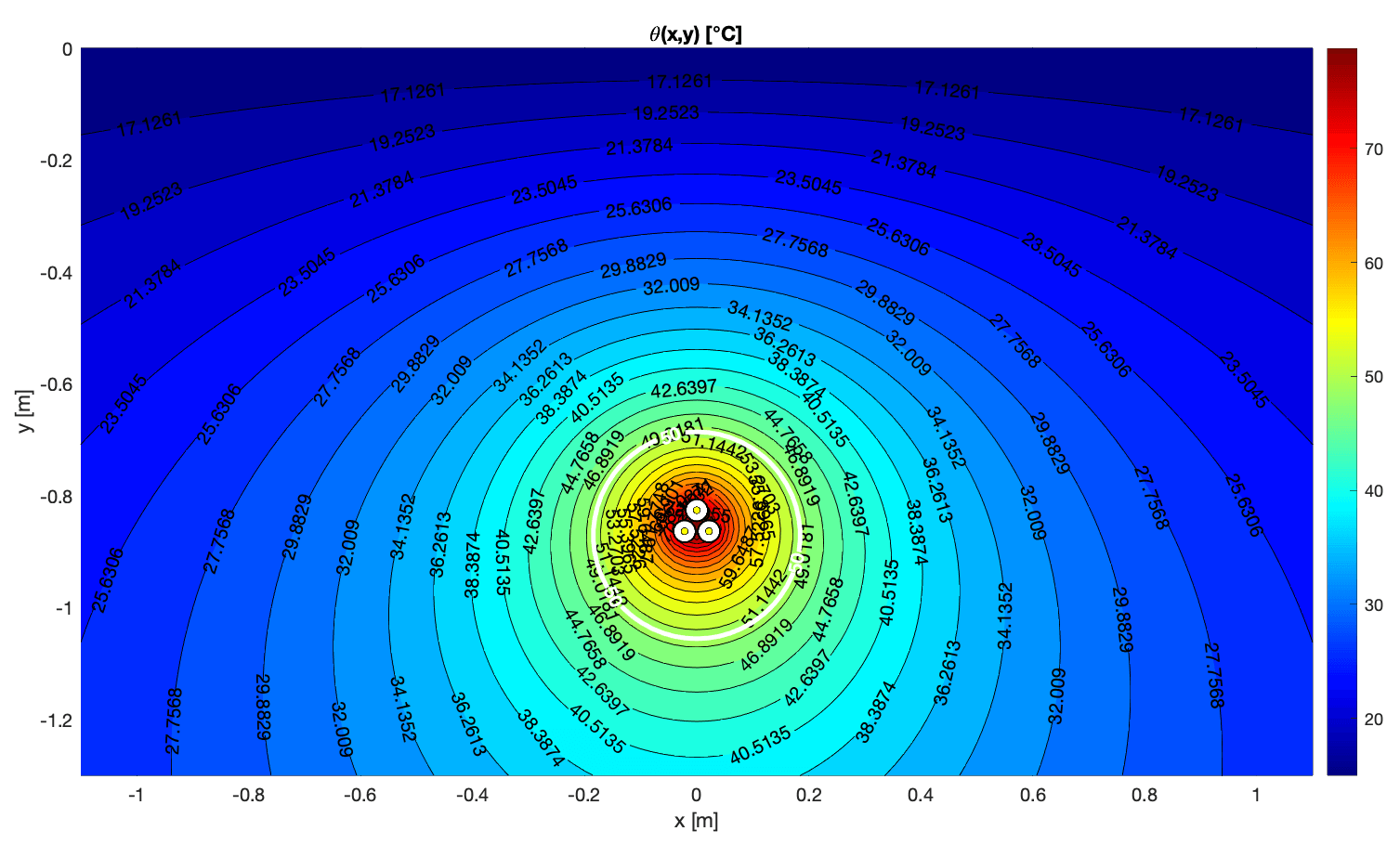
The resulting temperature field is shown:
| Heat field of cables | Heat field of equivalent heat source |
|---|---|
 |
 |
The temperature field using the finite element method is shown as follows, however contour lines cannot be drawn:

The temperature field can be calculated and visualized simply by the use of a simple Matlab program.
% heat_field.m
% Temperature field of buried line sources in semi-infinite soil
% Semi-infinite half-space with isothermal surface at y = 0.
% Cables are infinite line sources at (x_k, y_k), y_k < 0.
clear; close all; clc

%% ------------------------------------------------------------------------
%  Parameters
% -------------------------------------------------------------------------
theta_a  = 15;       % ambient / surface soil temperature [°C]
rho_soil = 1;        % soil thermal resistivity [K*m/W]  (adjust!)
con      = 0;        % counter for number of cables
theta_highlight = 50 % contour line to highlight [°C]

%% ------------------------------------------------------------------------
%  Define cable system (example)
%  para(k,:) = [x_k, y_k, W_k, diam_k]
%  x_k, y_k in m  (y_k < 0 below surface), W_k in W/m, diam_k in m
% -------------------------------------------------------------------------
diam = 0.0415;   % cable diameter [m]

x1 =  0.0;    y1 = -0.8259; W1 = 32.805;
x2 = -0.0218; y2 = -0.8636; W2 = 32.840;
x3 =  0.0218; y3 = -0.8636; W3 = 32.840;
con = con + 1; para(con,:) = [x1, y1, W1, diam];
con = con + 1; para(con,:) = [x2, y2, W2, diam];
con = con + 1; para(con,:) = [x3, y3, W3, diam];

%% ------------------------------------------------------------------------
%  Field grid
%  x: horizontal; y: depth (0 = surface, negative downward)
% -------------------------------------------------------------------------
x_min = -1.1; x_max = 1.1;  dx = 0.02;
y_min = -1.3; y_max = 0;  dy = 0.02;

xp   = x_min:dx:x_max;
yp   = y_min:dy:y_max;

nx = numel(xp);
ny = numel(yp);

theta = theta_a * ones(ny, nx);   % initialize with ambient temperature

%% ------------------------------------------------------------------------
%  Compute temperature field
% -------------------------------------------------------------------------
for i = 1:ny
    for j = 1:nx
        dT = deltatheta_1P(xp(j), yp(i), para, rho_soil);
        theta(i,j) = theta_a + dT;
    end
end

%% ------------------------------------------------------------------------
%  Plot
% -------------------------------------------------------------------------
figure('position',[100,100,900,700]);
hold on; box on; grid on
colormap(jet);

% contour plot of temperature
[C,h] = contourf(xp, yp, theta, 30);  % 30 levels
clabel(C,h);
colorbar;
xlabel('x [m]');
ylabel('y [m]');
title('\theta(x,y) [°C]');

% --- WHITE HIGHLIGHT CONTOUR AT theta_highlight --------------------------
[Chigh, hhigh] = contour(xp, yp, theta, ...
    [theta_highlight theta_highlight], ...  % single contour level
    'LineColor','w', 'LineWidth',2.5);
% optional label on highlighted contour:
clabel(Chigh, hhigh, 'Color','w', 'FontWeight','bold');

% draw cables as circles
for k = 1:con
    xk   = para(k,1);
    yk   = para(k,2);
    diam = para(k,4);
    rectangle('Position',[xk - diam/2, yk - diam/2, diam, diam], ...
              'Curvature',[1 1], 'FaceColor','k');
    rectangle('Position',[xk - 0.45*diam, yk - 0.45*diam, 0.9*diam, 0.9*diam], ...
              'Curvature',[1 1], 'FaceColor','w');
    rectangle('Position',[xk - 0.15*diam, yk - 0.15*diam, 0.3*diam, 0.3*diam], ...
              'Curvature',[1 1], 'FaceColor','y');
end

set(gca,'YDir','normal');   % depth increasing downward
axis equal tight;

%% ========================================================================
%  Local function: temperature rise at a single point (x,y)
% ========================================================================
function dT = deltatheta_1P(xp, yp, sources, rho_soil)
% dT = temperature rise above ambient at point (xp,yp)
% sources: [x_k, y_k, W_k, diam_k]
%
% Semi-infinite domain with boundary at y=0 (isothermal).
% Real source at (x_k, y_k), image source at (x_k, -y_k).
% Formula: dT = rho_soil/(2*pi) * sum_k W_k * ln(r_img / r_src)

    xk = sources(:,1);
    yk = sources(:,2);
    Wk = sources(:,3);
    dk = sources(:,4);   % diameter [m]

    N  = size(sources,1);
    sumW = 0;

    for k = 1:N
        dx    = xp - xk(k);
        r_img = sqrt(dx.^2 + (yp + yk(k)).^2);   % distance to image
        r_src = sqrt(dx.^2 + (yp - yk(k)).^2);   % distance to real source

        % avoid log(0) at the cable center: clip r_src to at least cable radius
        r_min = max(dk(k)/2, 1e-6);              % 1e-6 m fallback
        r_src = max(r_src, r_min);

        sumW = sumW + Wk(k) * log(r_img ./ r_src);  % MATLAB uses log = ln
    end

    dT = rho_soil / (2*pi) * sumW;
end
We have been asked to explain once more why our result differs from Cymcap.
Comparing calculation reports between Cableizer and Cymcap is genuinely difficult because their software is essentially a black box. Cableizer, on the other hand, operates with radical transparency: full public documentation, accessible to anyone, containing not just parameters and explanations but every formula exactly as implemented in the calculations.
Our service includes blog posts like this here where we even provide the reader with working code to verify our claims and results. Do you get this kind of transparency from your other software provider?
Anyways, we are not going to repeat the full analysis here but you find an extensive and interesting article on LinkedIn with the background story and the full analysis. Enjoy ;-)