Based on two example arrangements it is described how buried systems in backfills are modelled and simulated in Cableizer (introduced 2020-08-25).
Posted 2020-08-25
Categories:
New feature
, Theory
With the software version deploy from 2020-08-25, a new method to consider backfill areas when calculating the approximated temperature field was introduced.
Based on two example arrangements it is described how buried systems in backfills are modelled and simulated in Cableizer. Some uncertainties of this new analytical method for buried systems are also discussed. Compared to the previous method and the IEC method - it is unclear if the IEC method is at all as generally applicable as the proposed method which allows for different backfills and multiple differently loaded cable systems and heat sources - this new analytical method changes how the number of loaded objects in the backfill is interpreted and how the calculation of the temperature rise of a system due to other sources is calculated.
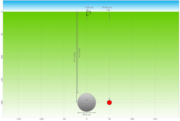
The example arrangements consist of a system A with 3 single-core cables that are loaded with 400 A and an unloaded (0.001 W) heat source (system B) located at a distance of 50 cm from the centre of system A, allowing us to obtain the temperature at that position. In the first arrangement, the cables are laid in a common plastic duct, while in the second arrangement, the cables are directly laid in the concrete in a flat arrangement with a spacing of 5 cm between cables.
In the first arrangement, both the cable system and the heat source are situated in a rectangular backfill, while in the second arrangement, only the cable system is situated in a round backfill. The thermal resistivity of the backfill $\rho_b$ has been selected as 6.0 (intentionally high for illustrative purposes), while the thermal resistivity of the soil $\rho_4$ was chosen as 1.5.
| Arrangement |  |
 |
Calculation of the thermal resistance of the soilSince system A is embedded in concrete, its thermal resistance to ambient $T_{4iii}$ is calculated assuming a uniform medium having the thermal resistivity equal to the concrete $\rho_b$. The same method can be applied for the calculation of the thermal resistance $T_{4iii}$ for the heat source in the first arrangement (calculation steps are not detailed here), while the calculation for the directly buried heat source in the second arrangement is done by using the thermal resistivity of the soil $\rho_4$.The substitution coefficient $u$ depends on the depth of laying $L_{cm}$ which is 200 cm in both cases, and the outer diameter $D_{o}$ which is 20 cm for the duct and 4.9 cm for the cable. The mutual heating coefficient $F_{mh}$ is 1.0 for the first arrangement since the cables are in a common duct, and needs to be calculated for the second arrangement. | ||
| $u = \frac{2L_{cm}}{D_o}$ | $\frac{400}{20} = 20.0$ | $\frac{400}{4.9} = 81.7$ |
| $F_{mh} = \prod_{k=1}^{q}\frac{d_{pk1}}{d_{pk2}}$ | 1.0 | middle phase: $\frac{\sqrt{9.9^2+400^2}}{9.9}^2 = 1633.5$ outer phases: $\frac{\sqrt{9.9^2+400^2}}{9.9}\cdot\frac{\sqrt{19.8^2+400^2}}{19.8} = 817.5$ |
| $T_{4iii} = \frac{\rho_b \mathrm{ln}(F_{mh}(u+\sqrt{u^2-1}))}{2\pi}$ | $\frac{6\mathrm{ln}(20+\sqrt{20^2-1})}{2\pi} = 3.52$ | middle phase: $\frac{6\mathrm{ln}(1633.5\cdot(81.7+\sqrt{81.7^2-1}))}{2\pi} = 11.93$ outer phases: $\frac{6\mathrm{ln}(817.5\cdot(81.7+\sqrt{81.7^2-1}))}{2\pi} = 11.27$ |
| Subsequently, a correction of the thermal resistance due to the backfill $T_{4db}$ is calculated for system A. The geometric backfill factor $G_b$ can be calculated in different ways (the method from IEC 60287-2-1 Ed.1.2 is used in this example) and depends on the backfill substitution coefficient $u_b$. The later depends on the vertical center of the backfill $L_b$ (which is identical for both arrangements) and the equivalent radius of the backfill $r_b$. For a round backfill, the equivalent radius is equal to the radius of the backfill, while an equivalent radius can be calculated from the dimensions of a rectangular backfill (this is left as an exercise to the reader). The number of loaded objects in the backfill $N_b$ is also a required input, and only objects of the same system are considered. It is 1.0 for cables in a common duct or when the mutual heating coefficient $F_{mh} = 1$ (i.e. the objects are treated as different sources), or equal to the number of sources $N_c$ otherwise. | ||
| $u_b = \frac{L_b}{r_b}$ | $\frac{200}{55} = 3.64$ | $\frac{200}{20} = 10.00$ |
| $G_b = \mathrm{ln}(u_b+\sqrt{u_b^2-1})$ | $\mathrm{ln}(3.64+\sqrt{3.64^2-1}) = 1.97$ | $\mathrm{ln}(10+\sqrt{10^2-1}) = 2.99$ |
| $N_b$ | 1 | 3 |
| $T_{4db} = \frac{G_b N_b (\rho_4-\rho_b)}{2\pi}$ | $\frac{1.97(1.5-6)}{2\pi} = -1.41$ | $\frac{2.99\cdot3(1.5-6)}{2\pi} = -6.43$ |
| Finally, the effective steady-state thermal resistance of the soil $T_{4ss}$ can be calculated. Please note that the large difference in the effective thermal resistance between the two arrangements is due to the fact that in the first arrangement, the number of conductors are combined ($n_{cc}$ = 3), while every cable is calculated separately in the second arrangement ($n_{cc}$ = 1). | ||
| $T_{4ss} = T_{4iii} + T_{4db}$ | $3.52-1.41 = 2.11$ K.m/W | middle phase: $11.93-6.43 = 5.50$ K.m/W outer phases: $11.27-6.43 = 4.84$ K.m/W |
Calculation of the temperature rise of the heat source due to other sourcesThis section explains how the temperature rise of the heat source caused by the cable system is calculated, considering that the cable system is located in a backfill. Of course, Cableizer does also calculate the temperature rise from the heat source on the cable system, but this calculation is not detailed here (in this case it is negligible due to the low losses in the heat source).The temperature rise by other buried objects $\Delta\theta_p$ is calculated differently for the two arrangements. In the first arrangement, the heat source is in the same backfill as the cable system, and the cable system is in a common duct, thus considered as a single buried object represented by a single temperature rise by buried object $\Delta\theta_{kp}$. In the second arrangement, the heat source is outside of the backfill of the cable system, and the three phases of the cable system are considered individually by three different $\Delta\theta_{kp}$. | ||
| $\Delta\theta_p = \sum_{k=1}^{q}\Delta\theta_{kp}$ $= \sum_{k=1}^{q} \frac{W_{tot}\rho_4\mathrm{ln}(d_{pk1}/d_{pk2})}{2\pi}$ |
$\frac{33.5\cdot1.5\mathrm{ln}(\sqrt{400^2+50^2}/50)}{2\pi} = 16.7$ K | middle phase: $\frac{11.3\cdot1.5\mathrm{ln}(\sqrt{400^2+50^2}/50)}{2\pi} = 5.6$ K left phase: $\frac{14\cdot1.5\mathrm{ln}(\sqrt{400^2+59.9^2}/59.9)}{2\pi} = 6.4$ K right phase: $\frac{13.5\cdot1.5\mathrm{ln}(\sqrt{400^2+40.1^2}/40.1)}{2\pi} = 7.4$ K total: 19.4 K |
| In the first arrangement, both the cable system and the heat source are embedded in the same concrete (backfill). Therefore, the temperature rise by buried object $\Delta\theta_{kp}$ is adjusted with the difference between the thermal resistivity of the backfill material $\rho_b$ and the thermal resistivity of the soil $\rho_4$: $\Delta\theta_{kp} = \Delta\theta_b + (\Delta\theta_{kp} - \Delta\theta_b) * \rho_b / \rho_4 = 14.7 + (16.7 - 14.7) * 6 / 1.5 = 22.7$, where $\Delta\theta_b$ is the temperature rise of the cable system in the middle on the top border of the backfill: $\Delta\theta_b = \frac{33.5\cdot1.5\mathrm{ln}(\sqrt{350^2+25^2}/\sqrt{50^2+25^2})}{2\pi} = 14.7$ K With this method, the difference in temperature rise inside the backfill due to the difference in thermal resistivity is taken into consideration. However, the calculation of $\Delta\theta_b$ is somewhat arbitrary and might not be the most suitable solution depending on the shape of the backfill and the position of the sources within the backfill. For a more accurate solution, it most probably would be necessary to model the soil with finite elements. Finally, the temperature of the heat source $\theta_{hs}$ can be calculated as: | ||
| $\theta_{hs} = \theta_a + \Delta\theta_p$ | 20 + 22.7 = 42.7 °C | 20 + 19.4 = 39.4 °C |
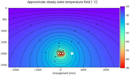
| The approximate steady-state temperature field graph has been modified with the same method and as expected shows a good agreement with the calculated temperatures of the heat source for both arrangements. It is clearly visible that the temperature rise inside the backfill is larger than outside, due to the larger thermal resistivity in the backfill $\rho_b$ as compared to the surrounding soil $\rho_4$. | ||
| Temperature field | 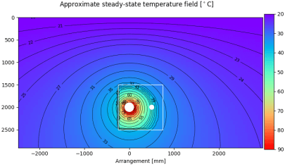 |
 |