This calculator provides you with a tool to calculate the conductor resistance using Bessel functions of first order to calculate the skin effect.
Posted 2026-01-01
Categories:
Tools
Skin effect in solid round circular conductors and proximity effects between solid round circular conductors were deeply investigated, specially by A.H.M. Arnold, and formulae were worked out for $y_s$ and $y_p$, through tedious calculations to approximate the Bessel's functions involved in the solution of Maxwell's equations.
The equations in IEC 60287-1-1 provide results with an error rate of <3 % for frequencies up to 100 Hz. This calculator uses the exact Bessel functions of first order to calculate the skin effect also for high frequencies and all round stranded conductor sizes.
With our tool you can calculate the conductor resistance and visualize it over a range of conductor temperature for the given cross-sectional area, spacing and frequency.
The equations below are taken from the publications Stojanovic20171 and Morgan20132.
The dc density $J_{\mathrm{dc}}$ within an isothermal solid cylindrical conductor is uniform, and is given by
| $$J_{\mathrm{dc}}=\frac{I_{\mathrm{dc}}}{\pi r_s^{2}}$$ | (1), |
where $I_{\mathrm{dc}}$ is the total current, and $r_s$ is the radius of the conductor.
The resistance per unit length of the cable conductor for DC current versus temperature can be determined as
| $$R' = R_0'\left(1+\alpha(\theta-20)\right).$$ | (2) |
For AC current, there are skin and proximity effects, causing the resistance increasing. For determining AC resistance, in IEC 60287-1-1 the following relation is used,
| $$R = R'\left(1+y_s+y_p\right).$$ | (3) |
$y_s$ models influence of the skin effect
$y_p$ models influence of the proximity effect.
Skin effect
The ac density distribution $J(r)$ in a linear isolated solid cylindrical conductor carrying a current $I$ is given by:
| $$ J(r) = \frac{J_s J_0(mr)}{J_0(m r_s)} = \frac{mI}{2\pi r_s} \left[ \frac{\operatorname{ber}(mr)+j\,\operatorname{bei}(mr)} {\operatorname{bei}'(m r_s)-j\,\operatorname{ber}'(m r_s)} \right] $$ | (4) |
where $\operatorname{ber}$, $\operatorname{bei}$, $\operatorname{ber}'$, and $\operatorname{bei}'$ are Kelvin functions, $J_0$ is a Bessel function of the first kind and zero order, and $J_s$ is the current density at the surface of the conductor, and
| $$ m = \left[ \frac{2\pi f\,\mu_0\,\mu_r(I,f,\sigma,T)}{\rho(T)} \right]^{1/2} $$ | (5) |
The relative permeability of the conductor $\mu_r$ depends on the magnetic-field strength $H$ and, hence, on the current $I$, and on the frequency $f$, the tensile stress $\sigma$, and the temperature $T$. $\mu_0$ is the permeability of free space, and $\rho(T)$ is the temperature-dependent resistivity. In the case of a nonmagnetic solid cylinder, $\mu_r=1$.
With alternating current, the skin effect factor $k_s$, that is, the ratio between the ac and dc resistances for an isolated solid circular cylinder with radius $r_s$ and negligible capacitive current, is given by:
| $$ k_{\mathrm{s}} = \frac{R_{\mathrm{ac}}}{R_{\mathrm{dc}}} = \operatorname{Re}\left[ \frac{m r_s\,J_0(m r_s)}{2J_1(m r_s)} \right] = \frac{m r_s}{2} \left[ \frac{ \operatorname{ber}(m r_s)\,\operatorname{bei}'(m r_s) - \operatorname{bei}(m r_s)\,\operatorname{ber}'(m r_s) }{ \left(\operatorname{ber}'(m r_s)\right)^{2} + \left(\operatorname{bei}'(m r_s)\right)^{2} } \right] $$ | (6) |
For interval $0.3<r_c/\delta_c<3$ the following relations provide error less than $3\%$:
| $$ y_s=\frac{x_s^{4}}{192+0.8x_s^{4}}, \qquad x_s=15.9\cdot 10^{-4}\sqrt{\frac{f\,k_s}{R'}}. $$ | (7) |
For conductors with circular cross-section, for $x_s\le 2.8$, relation (7) is recommended (Note: Until 2014 previous expressions were used). For other interval it is:
| $$ y_s= \begin{cases} -0.136-0.0177x_s+0.0563x_s^{2}, & 2.8\le x_s\le 3.8,\\ 0.354x_s-0.733, & x_s>3.8, \end{cases} $$ | (8) |
Proximity effect
The current density in a finite circular cylinder carrying an ac $I_1$ is expressed close to an infinitesimal wire carrying a current $I_2$ in the form
| $$ J(r,\varphi) = \frac{I_1\,j\,m\,r_s\,J_0(jmr)}{2\pi r_s^{2}\,J_1(jm r_s)} + \frac{I_2\,j\,m\,r_s}{\pi r_s^{2}} \sum_{n=1}^{\infty} \frac{r^{n}J_n(jmr)\cos(n\varphi)}{s^{n}J_{n-1}(jm r_s)} $$ | (9) |
where $J_n(jm r_s)=\operatorname{ber}_n(m r_s)+j\,\operatorname{bei}_n(m r_s)$, $J_1$ is a Bessel function of the first kind and first order, $n$ is an integer, $r$ is the radius measured from the center line, $r_s$ is the radius at the surface, $s$ is the axial spacing, and $\varphi$ is the azimuthal angle.
Proximity effects are modeled in standard $\mathrm{IEC}\,60287\text{-}1\text{-}1$ with expression
| $$ y_p = \frac{x_p^{4}}{192+0.8x_p^{4}} \left(\frac{d_c}{a}\right)^{2} \left[ 0.312\left(\frac{d_c}{a}\right)^{2} + \frac{1.18}{ \dfrac{x_p^{4}}{192+0.8x_p^{4}}+0.27 } \right], \qquad x_p=15.9\cdot 10^{-4}\sqrt{\frac{f\,k_p}{R'}}. $$ | (10) |
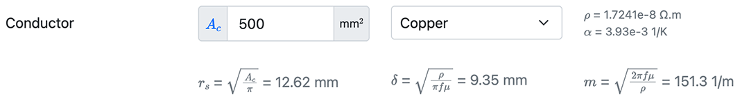
The cross-sectional area $A_c$ is an input between 0.5 mm2 and 1 600 mm2. Larger diameters are constructed using 4 to 7 segments – called Milliken – for which the equations used in this tool are not directly applicable. And the conductor material is selected from a drop-down list.
Based on the cross-sectional area of the conductor the diameter is calculated:
| $$r_s = \sqrt{\frac{A_c}{\pi}}$$ |
The selected conductor material defines the material parameters used in the equations:
The penetration depth $\delta$ can be calculated with following formula but is not needed directly:
| $$\delta = \sqrt{\frac{\rho}{\pi f \mu}}$$ |
Parameter $m$ is calculated:
| $$m = \sqrt{\frac{2 \pi f \mu}{\rho}}$$ |
With $r_s$, $\rho_c$ and $\alpha_c$ the DC resistance [$\Omega/m$] at operating temperature $\theta_c$ is calculated:
| $$R_{dc}=\left( \frac{\rho_c}{\pi r_s}\cdot 10^{-3} \right) \cdot (1 + \alpha_c (\theta_c - 20))$$ |
With $r_s$ and $m$ and equation (6) we can calculate the skin effect factor:
| $$ k_{\mathrm{s}} = \frac{R_{\mathrm{ac}}}{R_{\mathrm{dc}}} = \operatorname{Re}\left[ \frac{m r_s\,J_0(m r_s)}{2J_1(m r_s)} \right] $$ |
The proximity effect factor – which is typically less influential – we calculate using the equations from IEC 60287, given in (10). It requires additional input data, namely the center-center spacing between the phases. The outer diameter of the cable is required for input in order to check that the spacing is not defined too small.

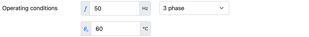
The operating condition is given by the system frequency $f$ and the conductor temperature under operation $\theta_c$. The selection of the number of phases influences the proximity effect $k_p$.
The output for the electrical resistance of the conductor is as follows:
| DC @ 20 °C | DC @ $\theta_c$ | $y_s$ | $y_p$ | AC @ $\theta_c$ |
|---|---|---|---|
| 0.04350 $\Omega/km$ | 0.05034 $\Omega/km$ | 0.06557 | 0.00792 | 0.05404 $\Omega/km$ |
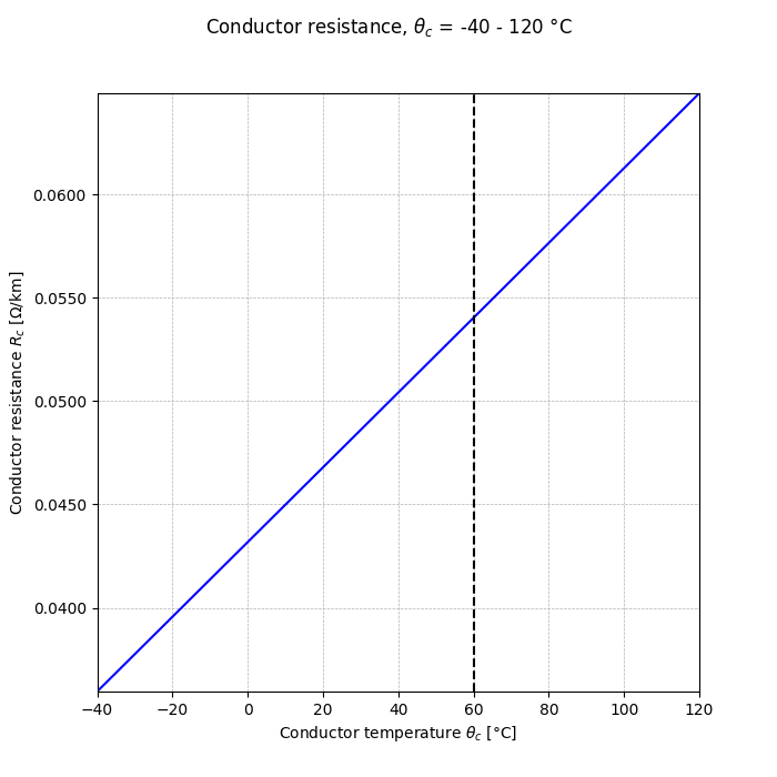
A plot is drawn which shows the conductor resistance over a range of conductor temperature for the given cross-sectional area, spacing and frequency:
The calculation is run over a range of cross-sections, spacings, and frequencies and the effect of these parameters is plotted.
| cross-section | spacing | frequency |
|---|---|---|
 |
 |
 |
1) Stojanovic, 'Self and Mutual Impedances of Power Cables', 2017
2) Morgan, 'The Current Distribution, Resistance and Internal Inductance of Linear Power System Conductors - A Review of Explicit Equations', 2013