We introduced a new postprocessing plot called "ECO" for economic optimization of power cables based on IEC 60287-3-2.
Posted 2026-02-13
Categories:
New feature
, User guides
The new image generator creates a single decision-focused chart: total cost over a range of conductor cross-sections at your selected operating point. It is intended for economic cable sizing: selecting a conductor size that is not only technically acceptable, but also economically justified over the cable’s service life.
IEC 60287-3-2 is directly about this topic: it “sets out a method for the selection of a cable size taking into account the initial investments and the future costs of energy losses during the anticipated operational life of the cable.”
In many engineering workflows, cable sizing is a two-step process:
The chart supports the second step: it makes the tradeoff visible between higher up-front cost (typically with larger conductors) and lower long-term loss cost (typically because electrical resistance decreases with increasing cross-section).
The x-axis shows a set of standardized conductor cross-sections around your selected/base value. This is important: the comparison stays within sizes you can actually specify and procure.
Y-axis: costs at the operating pointThe y-axis shows cost (typically displayed in k€) evaluated at the operating current shown in the axis label (for example: “Cost [k€] @ 235.0 A”). This means you are comparing sizes under the same operating condition.
The symbol of currency used, €, does not explicitly stand for the Euro but instead for any currency unit. Make sure that you use the same currency for all input data, for example convert the LME metal prices in USD to your currency unit.
Cu vs Al and cost componentsThe plot typically shows two material families (Cu and Al). Within each family, separate curves represent cost components such as:
This structure reflects the IEC intent: evaluate cable size by considering both initial investments and the future cost of energy losses over the anticipated operational life.
The generator highlights your current design choice as a base case marker on the relevant curves, based on:
A_cM_c (Cu or Al)This makes the chart practical for decision-making: you can immediately see whether moving one standard size up or down improves total cost under the same assumptions.
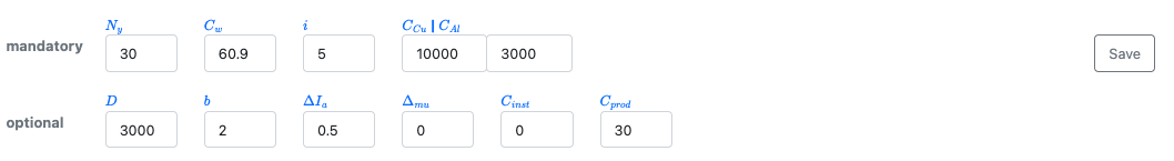
The chart is only as meaningful as its economic assumptions. The following inputs are taken from your ECO modal and control how investment and loss economics are evaluated.
| Parameter | Meaning (engineering interpretation) | Typical input guidance |
|---|---|---|
Ny[y] |
Years of operation (IEC example: 30) |
Anticipated operational life (years) used to accumulate loss economics over time. Commonly 20-50 years for many cable projects; set to your project life basis or to the governmental/corporate requirements for cost comparisons. |
Cw[€/MWh] |
Cost per megawatt-hour of energy at the relevant voltage level (IEC example: 60.9) |
Energy price (cost of electrical energy) used to convert electrical losses into an annual cost contribution. Use your tariff or internal energy valuation (often specified in $/kWh or €/kWh; the tool may use an equivalent base unit). |
i[%] |
Discount rate, excluding inflation (IEC example: 5.0) |
Discount/interest rate for life-cycle evaluation (present-worth / annuity effects over the operational life). Use your governmental/corporate/project discount rate. It is commonly a few percent to low double-digit, depending on policy. |
C_Cu[€/ton] |
LME price for copper (IEC example: n.a.) |
Copper cost parameter used by the investment model to represent the conductor material contribution for Cu designs. Use price from London Metal Exchange (LME) for 3-months-buyer or your internal procurement basis for copper (commodity price assumptions + fabrication adders as applicable).
This approach is different from IEC. |
C_Al[€/ton] |
LME price for aluminium (IEC example: n.a.) |
Aluminium cost parameter used by the investment model to represent the conductor material contribution for Al designs. Use price from London Metal Exchange (LME) for 3-months-buyer or your internal procurement basis for aluminium (commodity price assumptions + fabrication adders as applicable).
This approach is different from IEC. |
D[€/MWh] |
Annual demand charge (IEC example: 3000) |
This is the cost of additional supply capacity per year, depending on your economic model and accounting for the cost impact of supplying loss power capacity. It is utility- or project-specific. In sensitivity checks focused purely on energy losses, engineers set this to zero. |
b[%] |
Annual percentage increase in energy cost, excluding inflation (IEC example: 2.0) |
This represents the annual escalation for energy price assumptions, meaning how energy cost changes year-to-year in the evaluation model. Often zero up to a few percent depending on your forecast methodology. Use your internal assumption or contract basis. |
Delta_Ia[%] |
Annual percentage increase in load (IEC example: 0.5) |
May be chosen to be zero or corresponding the increase in current which reflects the increase in additional load being added to the grid which is being supplied by the cable under investigation. Make sure that the current at the end of the expected lifetime is no higher than the permissible load current of the cable; This is not automatically checked. |
Delta_mu[%] |
Annual percentage increase in the loss load factor (IEC example: 0) |
May be chosen to be zero or a small value. Ensure that the maximum value of $\mu$ at the end of the operating period does not exceed 1 or else the cable would be operated at higher load than it's rating was calculated; This is not automatically checked. |
C_inst[€] |
Total installation cost for the full system length $L_{sys}$ for the selected cable, in the study currency (IEC example: n.a.) |
The installation cost is assumed to be constant and independent of conductor type and size. In practice, it may be slightly higher for larger/heavier cables due to transport, pulling, and installation effort, or vice versa. These are purely installation-related cost component used in the investment model (labor, route-specific effort, accessories depending on your model), it is a project-specific number, typically derived from internal cost databases, contractor offers, or historical installations.
This approach is different from IEC. |
C_prod[€/m] |
Manufacturing cost per meter excluding the conductor metal cost, in the study currency (IEC example: n.a.) |
Project-specific; typically derived from vendor pricing or internal price curves. This value should include the cost of materials for screen, sheath, and armor, since these components are assumed to be largely independent of conductor cross-sectional area and are driven primarily by electrical requirements. For other cross-sections, a percentage adjustment is applied to reflect higher (or lower) manufacturing costs for larger (or smaller) conductors.
This approach is different from IEC. |
Let's show a simple example with two cable systems with three single-core cables 20 kV with 240mm2 Al in touching trefoil arrangement in a burial depth of 85 cm.
| Arrangement with two cable systems in trefoil |
|---|
 |
The ambient temperature $\theta_a$ is 15°C, the thermal resistivity of the soil is $\rho_4$ is 1.0 K.m/W
For the economical input data the example values from IEC 60287-3-2 were used as far as possible.
The calculation was done for two different current ratings, the higher the rating the greater the losses and the more likely a larger cross-section or a switch to copper instead of aluminium can be.
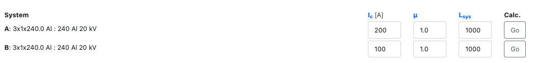
The resulting economic optimization plot with the losses over a range of conductor cross-sections is shown for two different currents:
| 200 A | 100 A |
|---|---|
 |
 |