We introduced a finite element method to calculate the temperature fields.
Posted 2022-04-06
Categories:
New feature
, Plots
, Theory
With the new version from March 2022, we provide two methods to calculate the approximated temperature field (ATF) for buried cables: The superposition principle and the Finite Element Method.
The original method to produce the approximated temperature field (ATF) for buried cables is based on the superposition principle. The temperature distribution is calculated assuming that the cables are directly buried in soil with a constant thermal resistivity $\rho_4$, that the heat loss $W_k$ is located in the center of cable or heat source $k$, and that the soil surface forms an isothermal at ambient temperature $\theta_a$.
$$\theta(x,y)=\theta_a+\frac{\rho_4}{2\pi}\sum\limits_{k=1}^N \left\{W_k\ln\left(\frac{\sqrt{(x-x_k)^2+(y+y_k)^2}}{\sqrt{(x-x_k)^2+(y-y_k)^2}}\right)\right\}$$
The temperature distribution does estimate the influence of the thermal resistivity of backfills $\rho_b$ if applicable. And in case of partial soil drying-out, the critical soil temperature $\theta_x$ is highlighted in red in the temperature field.
With the new version from March 2022, a second method was introduced to calculate the approximated temperature distribution in the soil for buried, subsea, tunnels and for the first time even for troughs. This new method is using the finite elements to calculate the heat distribution through conduction using the calculated conductor temperatures as boundary condition.
| ATF with colormap coolwarm | Mesh field |
|---|---|
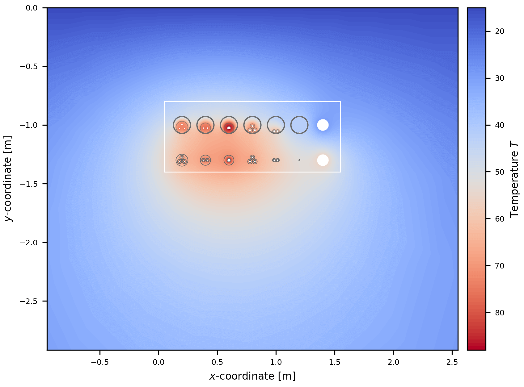 |
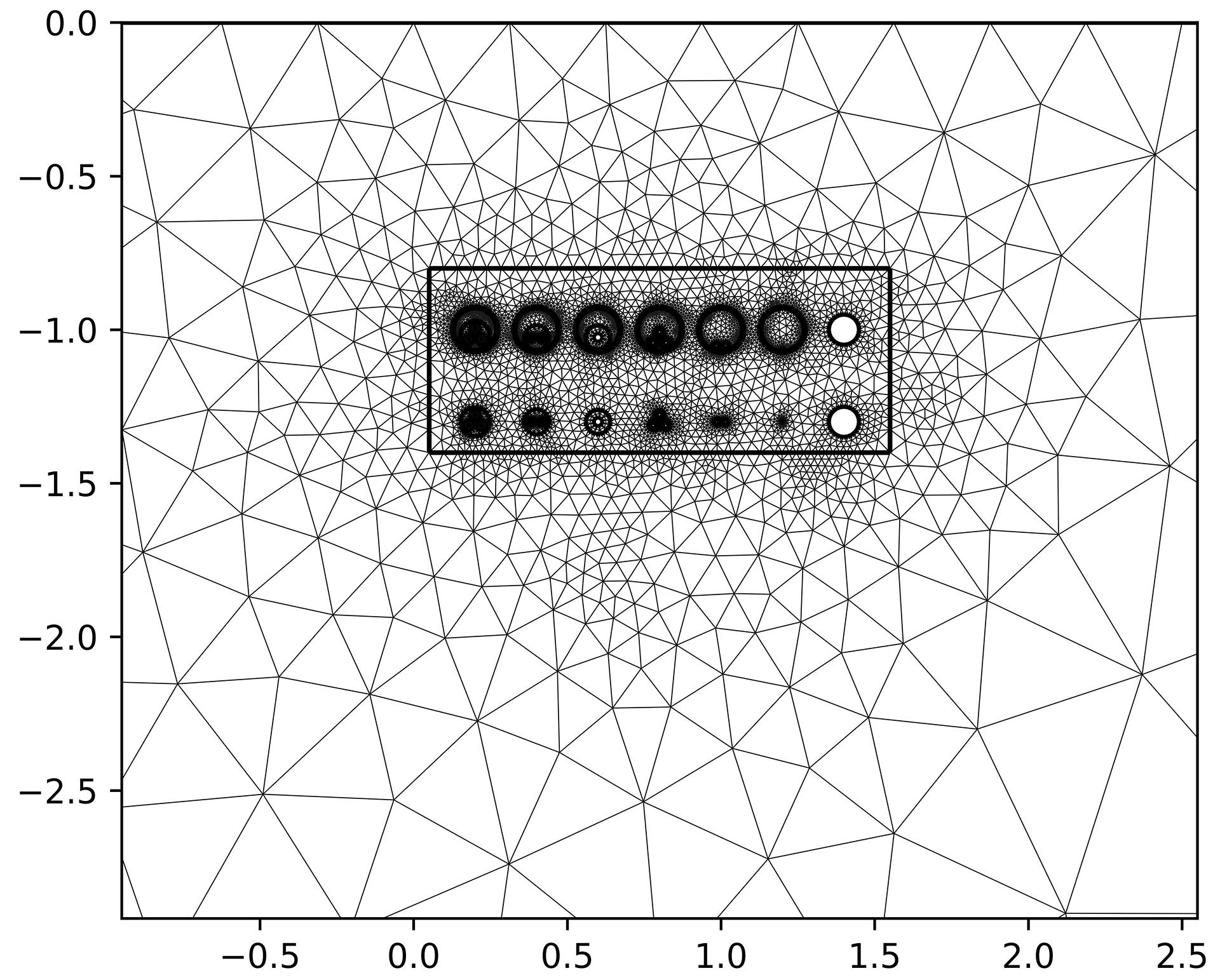 |
The extensive python FEM module PyGimli is used for all our applications using the finite element method, including the calculation of the temperature distribution. Thanks to the contributors of PyGimli.
The radio selector to choose finite element method to create the ATF had been there since mid December 2021, but except for very simple installations, it was unfortunately not working properly yet. The now deployed version is working stable in all tested cases.
Following definitions of the finite element model apply:
The following images show how the geometry is defined within a world with a range of 20 m to the sides and below.
| ATF of world geometry | Mesh field of world geometry |
|---|---|
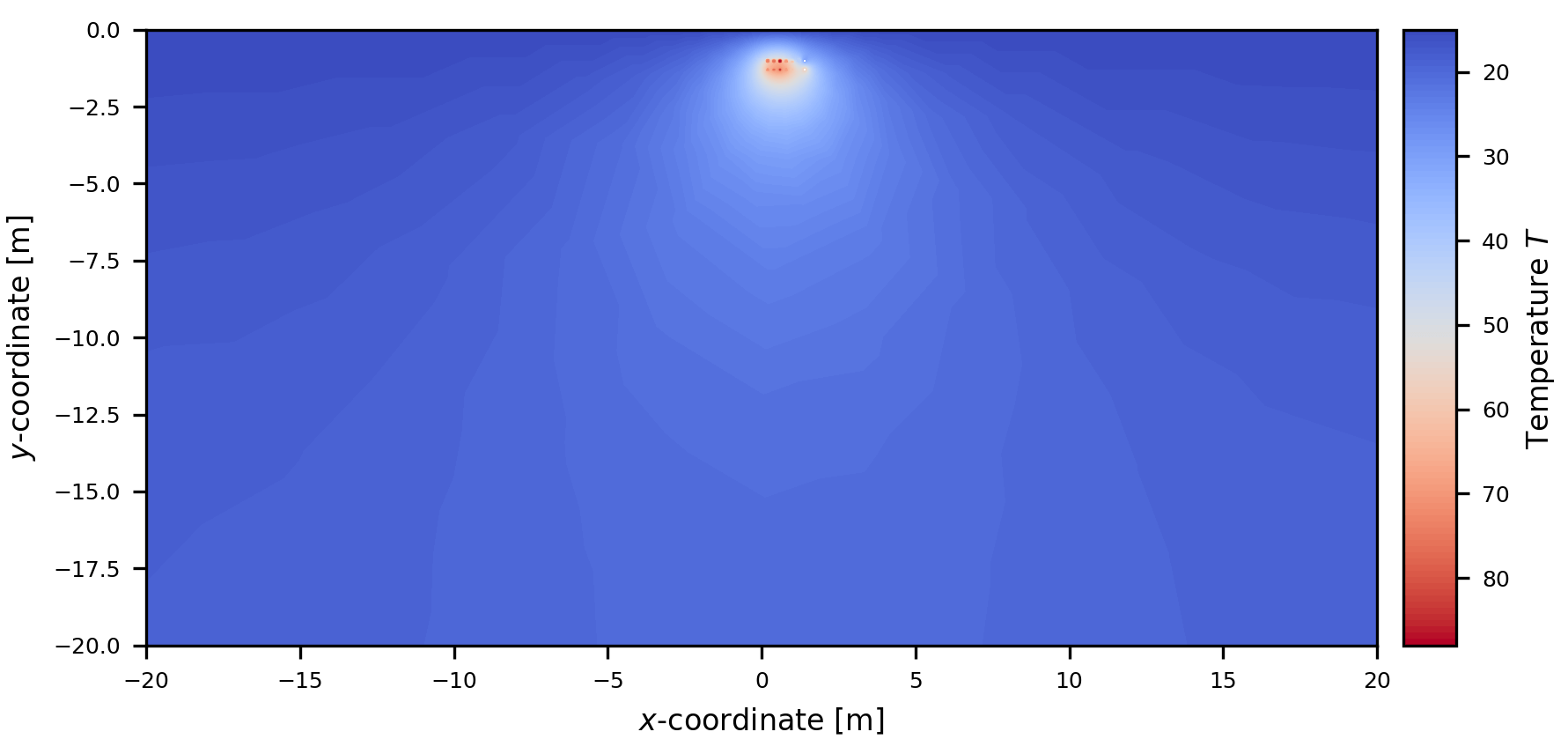 |
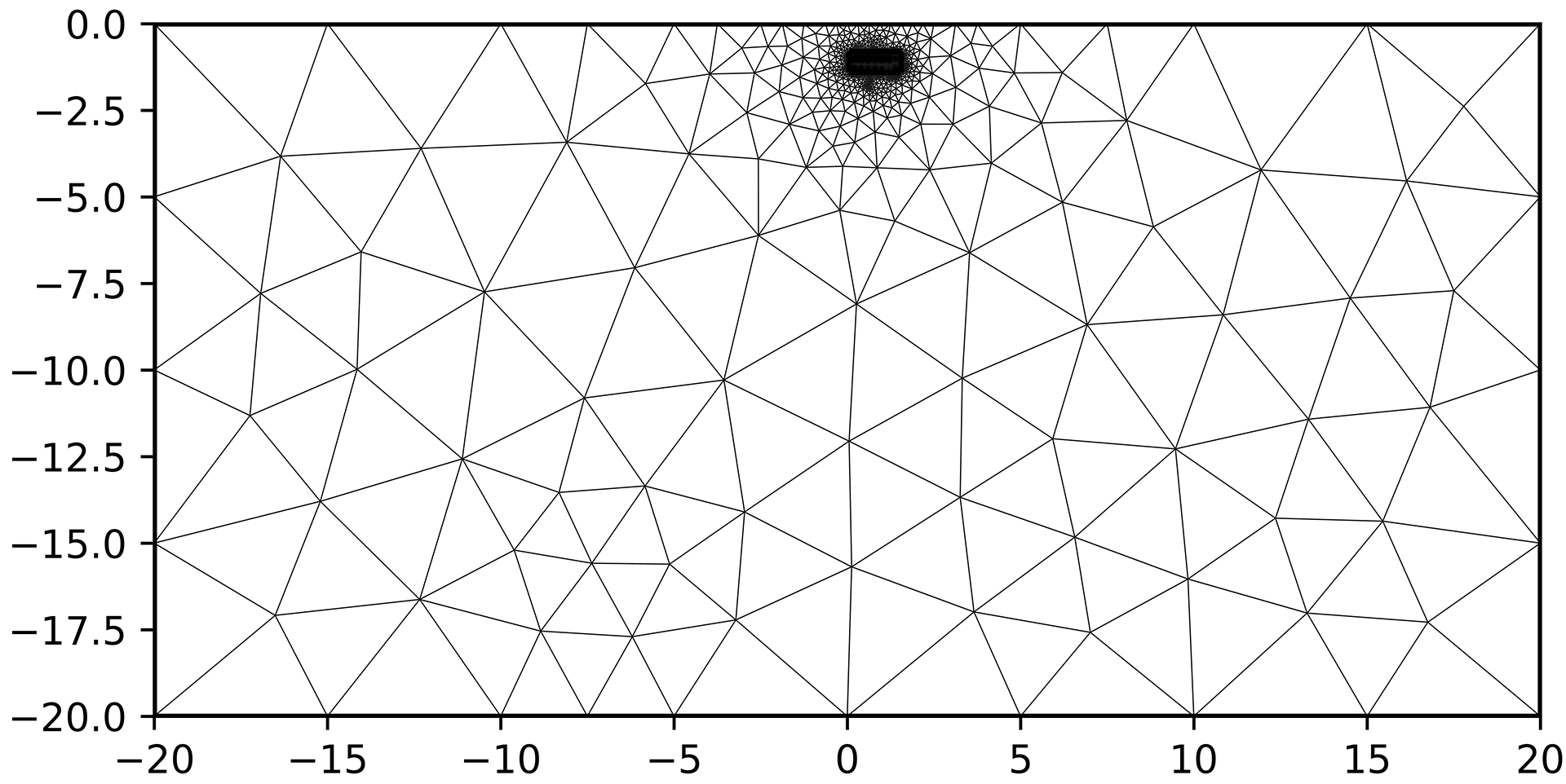 |
This new method comes with following features which will provide a fantastic user experience.
Limitations are:
Following plots show fine details of the plot and the mesh field. This shall bear witness to the outstanding properties of this new method.
| Details of the ATF with colormap plasma | Detailes of the mesh field |
|---|---|
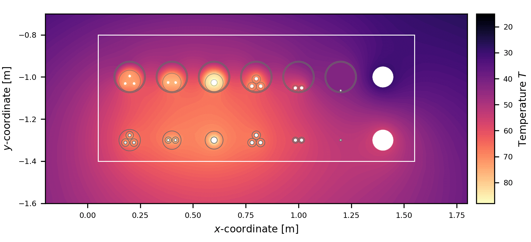 |
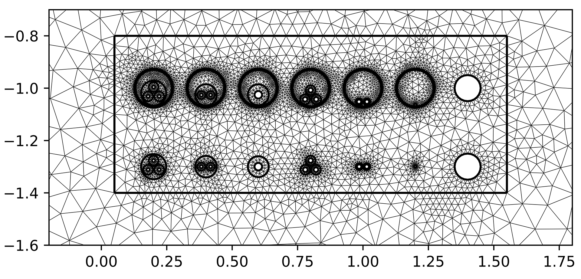 |
Based on the implemented finite element method for ATF, we will introduce the possibility to do the thermal rating calculation using FEM for buried cables. This feature will come in the near future and will allow the users to accurately consider the effect of non-homogenous environment.