Cableizer calculates the magnetic fields of multiple systems with different frequencies and load-flow directions. The magnetic field strength is diagrammed as impressive and meaningful two-dimensional color-map with contours of selected values and additionally in the classic, simple one-dimensional distribution over ground. Once more, this great new feature has been included without additional costs for our customers.
Posted 2016-02-22
Categories:
New feature
, Plots
, Theory
, User guides
Everyday we use electrical appliances and devices and wherever electricity is used, electromagnetic fields are created. Electric fields occur as soon as an appliance is connected to the power supply and the current flow gives rise to a magnetic field. The electric field is completely shielded by the cable sheath and the soil. This means that no electric field is detectable even if we are standing directly above the underground cables. The magnetic fields, however, freely penetrate practically all materials, and screening is therefore only possible with the aid of special metal alloys and even then only to a limited extent.
With underground cables, the conductors are very well insulated and can therefore be placed close together, as a result of which the reach of the magnetic fields is reduced. This means that, compared with overhead power lines carrying the same current, the magnetic field of an underground cable system has a much smaller spatial extension. Although the exposure may be just as high directly above an underground cable system as it is immediately beneath an overhead power line, it decreases more quickly on departing laterally than is the case with overhead lines.
Cableizer calculates the magnetic fields of multiple systems with different frequencies and load-flow directions. The user can add a phase shift for each system, interesting for non-synchronous systems. Each system can also be deactivated for the calculation of the magnetic field, interesting if regulations state that certain systems can be neglected (e.g. in Switzerland, 3 phases in the same pipe). All this has been released and added to your existing account without any additional costs.
The peculiarities of the different possible power systems are fully covered. Unlike other tools, it calculates the magnetic field of 16.7 or 50 Hz 1-phase AC system with 2 wires, which is used by railway transmission systems correctly. So for example, you can calculate a 1.5 kV 1Ph DC system of the Dutch railway in parallel to a 20 kV 50 Hz 3Ph AC distribution system or two 110 kV 16.7 Hz 1Ph AC system of Deutsche Bahn in parallel to a 220 kV 50 Hz 3Ph AC systems of Tennet.
The magnetic field strength is diagrammed as impressive and meaningful two-dimensional color-map with contours of selected values in μT and additionally in the classic, simple one-dimensional distribution over ground.
The magnetic field depends not only on the current rating but also on the load-flow (direction of current) and the phase arrangement (position of the conductors). Multiple systems can lead to a compensation or an amplification of the magnetic field strength. The phase arrangement is set in the project editor and we are working on a function to automatically define the optimal phase arrangement for a predefined area.
Features:
The magnetic field is calculated based on the law of Biot-Savart where each sub-conductor is represented by a filament current extending along its axis. The strength of a magnetic field is proportional to the current and decreases as the distance from the source increases. It is not stopped by ground or buildings, trees, etc. The magnetic fields from different phases may tend to add together or cancel each other depending upon location of the phases and the direction of the load flow.
| The magnetic field strength is calculated at point [$x_k$, $y_k$] due to all current sources at all time steps |
|---|
| $$0.2\pi \sqrt{ 1/m_{EMF} \sum\limits_{j=10,10}^{j_{max}} { \left[ \sum\limits_{phases} {{H_x}^2} + \sum\limits_{phases} {{H_y}^2} \right] } }$$ |
| The x- and the y-components of the magnetic field at point [$x_k$, $y_k$] due to current source at [$x_1$, $y_1$] |
| $$- \frac{I_{EMF}}{\pi} \left(\frac{- y_{1} + y_{k}}{\left(- x_{1} + x_{k}\right)^{2} + \left(- y_{1} + y_{k}\right)^{2}} + \frac{2 p_{soil} + y_{1} + y_{k}}{\left(- x_{1} + x_{k}\right)^{2} + \left(2 p_{soil} + y_{1} + y_{k}\right)^{2}}\right)$$ $$\frac{I_{EMF}}{\pi} \left(- \frac{- x_{1} + x_{k}}{\left(- x_{1} + x_{k}\right)^{2} + \left(2 p_{soil} + y_{1} + y_{k}\right)^{2}} + \frac{- x_{1} + x_{k}}{\left(- x_{1} + x_{k}\right)^{2} + \left(- y_{1} + y_{k}\right)^{2}}\right)$$ |
| The current for each phase at the time step $t_{EMF}$ is given as follows |
| $$\begin{cases} \sqrt{2} I_{c} \cos{\left (\alpha_{f} + \omega t_{EMF} \right )}, & \text{3-phase system with relative phase angle 120°, phase R (L1)} \\ - \sqrt{2} I_{c} \cos{\left (\alpha_{f} + \omega t_{EMF} + \frac{\pi}{3} \right )}, & \text{3-phase system with relative phase angle 120°, phase S (L2)} \\ - \sqrt{2} I_{c} \sin{\left (\alpha_{f} + \omega t_{EMF} + \frac{\pi}{6} \right )}, & \text{3-phase system with relative phase angle 120°, phase T (L3)} \\ \sqrt{2} I_{c} \cos{\left (\alpha_{f} + \omega t_{EMF} \right )}, & \text{2-phase system with relative phase angle 180°, phase U (L1)} \\ - \sqrt{2} I_{c} \cos{\left (\alpha_{f} + \omega t_{EMF} \right )}, & \text{2-phase system with relative phase angle 180°, phase V (L2)} \\ \sqrt{2} I_{c} \cos{\left (\alpha_{f} + \omega t_{EMF} \right )}, & \text{Mono-phase system (L1)} \\ I_{c}, & \text{DC system, phase P (L1)} \\ - I_{c}, & \text{DC system, phase N (L2)} \\ \end{cases}$$ |
The calculation method was developed by Prof. Dr. Chamorel from the Federal polytechnical institute of technology in Lausanne (EPFL).
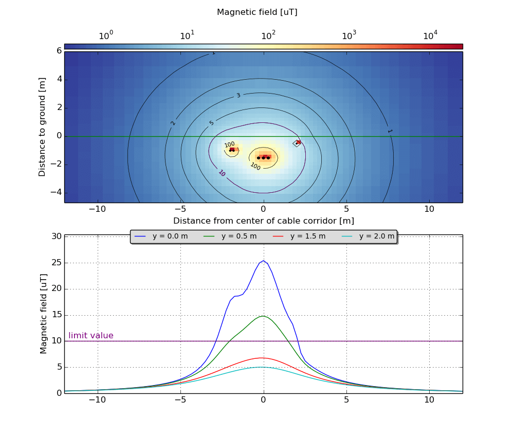
The following graph shows the magnetic field of a 380 kV 3-phase AC system with 50 Hz and 600 A, a 132 kV 1-phase system with 2 wires with 16.7 Hz and 400 A (as used by the Swiss Railway) plus a 1 kV 2-phase DC system with 0 Hz and 150 A. Note the emphasized 10 μT level of the magnetic field strength.
| Magnetic field of a 50 Hz, 16.7 Hz and a 0 Hz system |
|---|
 |