Cyclic loading

For the rating calculation of cyclic loading of buried cables two main methods are used:

1. The method according to IEC 60853 using the thermal capacity of the cable.
2. The Neher McGrath method using a load factor for the system.

Cableizer uses the method by Neher McGrath and allows the user to set a unique load factor for each cable system in the arrangement. In addition to the original method, one can change the transient period and select a soil diffusivity valid for the surrounding soil. In Cableizer, the characteristic diameter is not a constant but is calculated depending on the cable and its surrounding. Using a correct characteristic diameter is important for cables with large diameters and for cables in ducts, pipes, or even tunnels. Last but not least, the constant coefficient used to calculate the loss factor from the load factor can also be set by the user.

Generally, it can be said for both methods that they...

• are applicable to cables buried in the ground, either directly or in ducts.
• are not applicable for cables in air, because the conductor temperature follows changes in load current too quickly.
• are capable of dealing with all types of cables.
• use a sinusoidal load which varies cyclically over a 24 h period and the shape of each daily cycle is substantially the same (in Cableizer, the user can change this time period).
• the soil properties are assumed to be constant in both time and space.

Let's have a closer look at the two methods:

Method IEC 60853

Van Wormer developed a theory in 1955 to subdivide the insulation and surrounding soil into smaller entities so the temperature gradient within is small. In the 70's, Cigre introduced procedures for transient rating calculations based on a simplification of this theory using a two-loop network. By the end of the 80's, this procedure, called lumped capacitance method, resulted in the IEC standard 60853 consisting of three parts.

• Part 1 deals with cyclic rating factors for cables of voltages not greater than 30 kV where the internal thermal capacitance can be neglected.
• Part 2 gives methods for calculating cyclic rating factors for cables whose internal thermal capacitance cannot be neglected, which in general applies to cables with voltages greater than 30 kV. Part 2 does also provide a method for calculating the emergency rating for cables of any voltage.
• Part 3 is an extension giving a method for calculating the cyclic rating factor, for cables of all voltages, where partial drying out of the surrounding soil is anticipated.

Ladder Network

In order to determine the cyclic rating factors where the internal thermal capacitance cannot be neglected, it is necessary to calculate the transient temperature response of the cable and its environment. For this the use of an analogous lumped thermal constant circuit to represent the cables is needed which is different from the one in IEC 60287. The equivalent thermal network used in the IEC standard contains only thermal resistances $T$ and thermal capacitances $Q$. It is applicable only where time periods greater than about 1 h are involved, and therefore is not applicable for cables in air.

Equivalent cable network for transient response calculation (source: IEC 853-2)

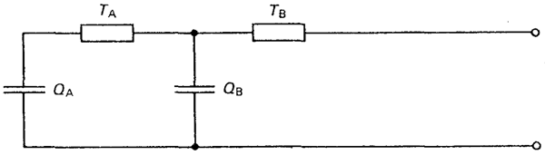The assumption is that the temperature distribution in the insulation follows a logarithmic distribution during the transient period. Depending on the duration of the transient, the ladder network needs to be adjusted. Whether a transient is short or long depends on the construction of the cable.

Thermal Capacitance

A thermal capacitance describes the ability to store heat and is defined by:

$Q = V · c$

where $V$ is the volume of the body in m³ and $c$ is the volumetric specific heat of the material in J/m³°C.

As an example, the thermal capacitance for a coaxial object with the internal diameter $D_1$ and external diameter $D_2$ such as a cable insulation is given by:

$Q = π/4 \left( D_2^2 - D_1^2 \right)c$

Influence of the soil

In order to calculate the transient temperature rise of the outer cable surface, the cable is represented by a line source in homogenous, infinite medium with uniform initial temperature and the earth surface being an isotherm. The temperature rise of the cable surface is calculated as follows with the function $Ei$ being the exponential integral:

$θ_e(t) = W_t ρ_s/4π \left[ -Ei \left(-D_e^2/16δt \right) + Ei \left(-L^2/δt \right) \right]$

Method Neher McGrath

Computation of a cyclic rating requires an evaluation of the cable capacitances and conductor temperatures at several time points. In 1957, Neher and McGrath proposed an alternative method which requires a modification of the external thermal resistance of the cable.

Loss factor

In order to evaluate the effect of a cyclic load upon the maximum temperature rise of a cable system, Neher observed that one can look at the heating effect of a cyclical load as a wave front that progresses alternately outward and inward in respect to the conductor during the cycle. He further assumed that with the total Joule losses generated in the cable equal to $W_I$, the heat flow during the loss cycle is represented by a steady component of magnitude $μW_I$, plus a transient component $(1-μ)W_I$ that operates for a period of time during each cycle with μ being the loss factor which is derived from the load factor $LF$.

Assuming that the temperature rise over the internal thermal cable resistance is complete by the end of the transient period $τ$, the thermal resistance to ambient $T_4$ may be written as:

$T_4 = μT_{4ss} + (1-μ)T_{4d}$

And the maximum temperature rise at the conductor may be expressed as:

$Δθ = W_I v_4 \left[ T_i + μ T_{4ss} + (1-μ) T_{4d} \right] + Δθ_d - θ_x$

where $T_i$ is the internal thermal resistance of the cable, $T_{4ss}$ is the external thermal resistance with constant load, and $T_{4d}$ is the effective transient thermal resistance in the earth. The effect of moisture migration is taken into account by two variables $v_4$ and $θ_x$. The transient component of the heat flow will penetrate the earth only to a limited distance from the cable, thus the corresponding thermal resistance $T_{4d}$ will be smaller than its counterpart $T_{4ss}$, which pertains to steady-state conditions.

Transient thermal resistance

Further, Neher assumed that the thermal resistance $T_{4d}$ may be represented with sufficient accuracy by an expression of the general form

$T_{4d} = Aρ_s \log{ \left( B \sqrt{ δτ } /D_e \right) }$

The length of the cycle or transient period $τ$ is expressed in hours and the soil diffusivity $δ$ is expressed in m²/s. The constants A and B were evaluated empirically to best fit the temperature rises calculated over a range of cable sizes. Using measured data, Neher obtained values for the constants A = 1/2 and B = 61200.

$T_{4d} = 0.5ρ_s \log{ \left( 61200 \sqrt{ δτ } /D_e \right) }$

Characteristic diameter

We introduce the following notation for a characteristic diameter $D_x$

$D_x = 61200 \sqrt{ δτ }$

The diameter $D_x$, at which the effect of the loss factor starts, is a fraction of the diffusivity of the medium δ and the length of the loss cycle τ. Inside the circle of this diameter, the temperature changes according to the peak value of the losses. Outside this circle, it changes with the average losses.

In Cableizer, the calculation of the characteristic diameter for a sinusoidal load is based on the IEEE paper 'Ampacity calculation for deeply installed cable' by E. Dorison, dated 2010. In the formulas presented in the paper, the cable diameter influences the diameter of the area affected by load variations. This is particularly important for cables in tunnels, where the tunnel diameter replaces the diameter of the cable. The calculation uses the modified Bessel function K of order zero $k_0()$ and the modified Bessel function of order one $k_1()$.

$D_x = D_{e} e^{\frac{2000}{D_{e} q_{x}} \operatorname{abs}{\left (\frac{\operatorname{k0}{\left (\frac{D_{e} q_{x}}{2000} \right )}}{\operatorname{k1}{\left (\frac{D_{e} q_{x}}{2000} \right )}} \right )}}$

Using the characteristic diameter, the thermal resistance to ambient can be written as:

$T_4 = ρ_s/2π \left[ μ \log{ (4L/D_e) } + (1-μ) \log{ (D_x/D_e) } \right] = ρ_s/2π \left[ μ \log{ (D_x/D_e) } + μ \log{ (4L/D_x) } \right]$

In the majority of cases, the soil diffusivity will not be known. In such cases, a value of 0.5 x 10^-6 m²/s can be used. This value is based on a soil thermal resistivity of 1.0 K.m/W and a moisture content of about 7% of dry weight. The value of $D_x$, for a load cycle lasting 24 hours and with a representative soil diffusivity of 0.5 x 10² m²/s is 211 mm (or 8.3 in).

Relationship between loss and load factor

Since decades, researchers have been searching for a relation between loss factor μ and the load factor LF. In engineering practice, the loss factor is approximated from the known or assumed load factor LF using an empiric equation.

$μ = (k)LF+(1-k)LF^2$

Some previous works have suggested the value k = 0.30 resulting in:

$μ = 0.3LF+0.7LF^2$

However, in Cableizer you can now set the constant coefficient k to any value between 0.04 and 0.40. And we give you a list of typical values which have been evaluated in different studies.

References:

• Ampacity Calculations for Deeply Installed Cables, E. Dorison et. al., IEEE Transactions on Power Delivery, Vol. 25, No. 2, April 2010